
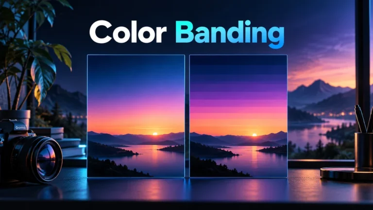
Color banding appears when a transition that should look smooth becomes visible tonal steps or stripes. It can arise from limited numerical precision, processing, compression, or the viewing path. A sky with bands is not automatically AI-generated. Compare the source and delivered version, identify where the steps first appear, and keep an unchanged reference before trying to soften them.
This guide focuses on tonal quantization, not a display buyer’s guide or a universal diagnosis. Its ramp and averaging exercise use original chosen values, not a photographed sky, measured monitor, or codec benchmark. They show why distinct shades can collapse into repeated levels and why a smoother derivative should not be called recovered source evidence.
A smooth transition can become a staircase
Imagine a broad wall that gradually becomes darker from one side to the other. In a smooth representation, nearby positions can differ subtly. If processing maps many nearby values to the same stored level, regions become flat until the next level begins. The boundary between those regions can appear as a band even though the underlying subject has no painted stripe.
Quantization is the numerical part of that example: a range of possible inputs is represented by a limited set of output values. It does not have to invent a new object to change the appearance. The output can retain the wall’s general shape while losing the fine tonal distinctions needed for a smooth transition.
Not every stripe is tonal banding. A shadow, physical paint line, light pattern, display interaction, or another processing effect can create stripes for different reasons. Describe the observation first: repeated boundaries across a gradual region. Do not infer a bit depth, encoder, or lighting frequency from appearance alone.
Also distinguish a static tonal pattern from a time-dependent light effect. Bands that change across camera rows or frames may need a different investigation. This article does not replace capture-light or sensor-timing troubleshooting. Its narrow question is how numerical shade steps become visible in a region expected to vary smoothly.
Bit depth describes precision, not the entire pipeline
Adobe’s bit-depth documentation explains the number of available values and distinguishes bits per channel from the total across RGB channels. For a simple unsigned channel, eight bits allow 256 codes. Do not confuse that single-channel count with the complete number of RGB combinations or with the number of visibly distinct shades on a particular screen.
More available codes can represent smaller numerical differences under a defined encoding, but a file’s final label does not reveal every prior stage. A higher-precision working file can contain material that was already quantized earlier. Moving it to a new format does not by itself recreate the original values that disappeared.
Keep numerical precision separate from spatial sampling. Reducing the density of color-channel sample locations is a different operation from reducing the values available at each location. A pipeline can do both. That distinction helps you avoid using “color depth” as a vague explanation for every soft colored edge or stepped gradient.
Metadata can support a representation description when it exposes the relevant field. It does not certify the entire history. The video metadata guide explains that wider limit. Record the format you actually inspected rather than assuming the camera, editor, and delivered copy all used it.
A four-level ramp makes quantization visible
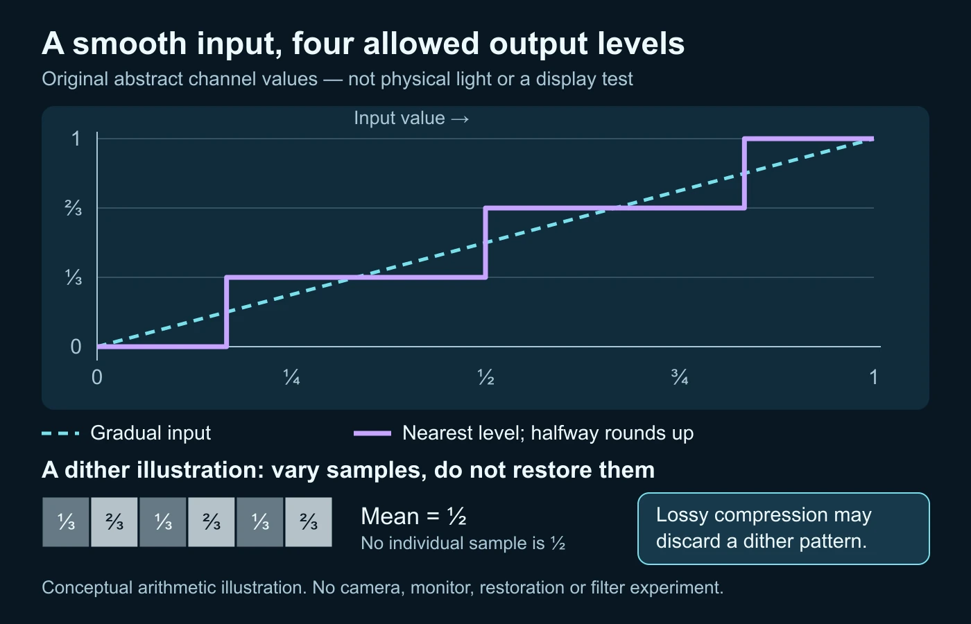
For an original arithmetic example, choose a normalized abstract channel ranging from zero to one. We sample it at equal intervals of one eighth. Then we restrict the output to four allowed values: zero, one third, two thirds, and one. These are teaching values, not a camera specification, color-space model, or recommended export setting.
Use a defined rule: multiply the input by three, round to the nearest whole number with halfway values rounded upward, and divide by three. The rule deliberately makes the steps obvious. It should not be assumed to describe an actual encoder’s complete quantization process.
| Input value | Four-level output | What happened |
|---|---|---|
| 0 and 1/8 | 0 | Two inputs share one output level. |
| 1/4 and 3/8 | 1/3 | Different shades become a plateau. |
| 1/2, 5/8, and 3/4 | 2/3 | The chosen halfway rule assigns 1/2 upward. |
| 7/8 and 1 | 1 | The final two inputs share the upper level. |
The repeated values are the important result, not the number of table rows. A region that had several gradual differences now contains runs of identical output. At a boundary, the value jumps to the next permitted level. Our diagram makes those plateaus visible without pretending that a natural sky contains exactly four shades.
Once only the quantized result remains, a plateau does not uniquely identify every original value. In this example, an output of one third can correspond to different selected inputs. A correction may estimate a smoother transition, but it cannot use the plateau alone to certify which input was present at each position.
Apply the reasoning carefully to real media. A video has multiple channels, defined transfer characteristics, noise, and other processing. The normalized arithmetic here is not a direct measurement of physical light or perceived brightness. It isolates one loss-of-distinction mechanism; the actual source and workflow still determine what happened to a real clip.
Dither trades a coherent boundary for variation
Dither can introduce small variations rather than leave a broad region at one uniform level. Adobe’s Illustrator gradient-dither guidance describes subtle noise to reduce visible steps in that feature. It is a specific artwork workflow, not proof that the same checkbox fixes every compressed video or display.
Use another chosen arithmetic example. Alternate one third and two thirds equally within a patch. Their arithmetic mean is one half, although none of those individual samples is one half. This explains how spatial variation can represent an average while keeping each allowed value discrete. It is not a universal perceptual formula or a reconstruction of unknown source pixels.
Inspect what the variation does to the task. A smoother-looking background may be useful for presentation, but added texture may be unsuitable for a technical comparison or a very clean graphic. Do not call the tradeoff invisible by definition. Review the actual delivery at its intended scale and preserve the unmodified source separately.
A source-specific limit matters here: FFmpeg’s gradfun documentation describes gradient interpolation and dithering for playback, and warns against using that filter before lossy compression because compression can discard the dither. That is not a universal command recommendation. No FFmpeg filter was executed for this article.
Compression and the viewing path can change the result
A gradient can pass through capture, editing, export, platform processing, playback, and display. A visible step in the final view therefore does not identify the first stage that created it. Keep copies and processing facts connected so you can compare the same region rather than blame the last application you opened.
The published compression-artifact guide discusses banding among broader delivery artifacts. Use it for the wider pattern vocabulary. This article’s contribution is the quantized-value explanation and a narrower gradient review, not another catalog of blocks, ringing, and motion smearing.
Viewing changes also complicate comparison. A screenshot captures one displayed result, potentially after scaling and other presentation changes. Do not treat it as the original numerical channel data. If practical, inspect the actual source and export with the same player and viewing size before interpreting a difference between two screenshots.
Keep display conclusions bounded. A pattern changing between viewing setups can motivate a viewing-path investigation, but it does not alone identify panel precision or a defective device. This guide provides no monitor calibration procedure, service-menu instructions, or hardware diagnosis. Use the actual product’s documented support when that is the unresolved question.
Banding and intentional posterization can look related
Posterization is useful supporting vocabulary when a creator deliberately reduces tonal variation for a graphic effect. Unwanted banding and deliberate tonal steps can therefore share visible characteristics. The appearance alone does not establish whether the reduction was accidental, intentional, or introduced later.
Ask what the creator intended and which version you have. An illustrated title card designed with broad flat regions should not be diagnosed as a failed natural gradient merely because it has boundaries. Conversely, an export that introduces new boundaries into a smooth project may warrant a delivery check even if someone likes the stylized result.
Keep style preference separate from evidence. A viewer may enjoy the posterized look, while a technical reviewer needs to know that tonal values changed. Describe the transformation and purpose when known. Do not silently turn “looks artistic” into permission to use the derivative as an unchanged source.
Compare a gradient without changing every condition
Start with one region and one question. Is the background distracting at normal viewing size, or are the steps affecting interpretation of a feature? Those are different tasks. Select a representative frame or short interval, keep an unchanged reference, and record the viewing scale before making a comparison.
Separate the recorded background from any added gradient graphic. They may enter the workflow at different stages. A smooth project graphic becoming stepped in delivery does not establish that the camera recorded a banded scene. A camera source already containing steps needs a different comparison from a newly generated background.
| Review item | Record | Limit to retain |
|---|---|---|
| Reference | Exact source or earliest usable copy. | An earlier repost may already be processed. |
| Region | Same gradient, frame, and viewing scale. | Different crops do not isolate a change. |
| Representation | Available precision and relevant format fields. | A final label is not the complete history. |
| Operation | Documented export or correction changed. | Multiple changes make attribution uncertain. |
| Task result | Viewing suitability or unresolved evidence. | Smoothness is not a source-detail certificate. |
When testing your own allowed workflow, change one relevant condition where the software actually permits it. Preserve the reference and record the real setting rather than copying a preset name from an unrelated application. If several properties change together, label the comparison combined rather than claim you isolated precision.
Inspect both the whole region and a stated close view. An enlarged crop can reveal boundaries that do not disturb the intended presentation. A tiny preview can hide boundaries important to the task. Show the relevant context so another reviewer can understand why the observation matters rather than selecting only its most dramatic appearance.
A fictional sky-background job, reviewed in branches
Imagine a team preparing a permitted educational clip with a broad dusk-sky region. It looks smooth in one working preview but striped in a delivery view. This is an invented job, not a camera shoot, export test, or measured quality comparison. The team needs to locate the difference without destroying the source.
First, the team opens the actual available source and the exact exported file at corresponding moments. If the steps are already present in the source, the export may not be the first affected stage. They record that finding instead of promising a new preset will recover the earlier gradient.
In another branch, the source and local export appear suitable in the same viewing path, but a platform view shows bands. The team records the platform copy and viewing conditions. That narrows the next question without pretending they know the service’s private encoder or the display’s exact behavior.
Now suppose a documented local export introduces the steps. The team can create a separate candidate addressing the relevant representation or processing choice, if supported. They compare the same sky and keep the source. This article does not assert which option will work or supply a measured improvement for that candidate.
If a correction makes the background smoother, the team examines what else changed. Did the fine texture become softer? Was visible noise added? Does the ordinary playback size still suit the project? A smoother crop is not the only acceptance condition, and a polished derivative should not replace the reference used to understand the problem.
Finally, the team records a narrow decision: suitable delivery for this presentation, source remains banded, change appears only in the observed viewing path, or cause remains unresolved. None of those outcomes requires claiming the scene was AI-generated. The worksheet makes the next check explicit while leaving unsupported history unknown.
A new representation is not recovered ground truth
Return to the four-level exercise. If a tool fills intermediate values between plateaus, several smooth curves could fit the available steps. Choosing a pleasant curve does not establish which original samples were lost. The correction can be useful, but its inferred values should remain a described processing contribution.
For a factual review, compare conclusions from the preserved source rather than quietly substituting the smoothed result. A candidate may help a person discuss the region, yet it can change the details that another examiner would inspect. Label the operation and retain the source relationship.
If better original material becomes available, it may answer a question the processed copy cannot. That is a new evidence source, not proof that the earlier correction was right. Keep corroboration and enhancement separate so your final explanation shows where a finding actually came from.
Choose a correction for its purpose and tradeoffs
For a gradient graphic you author, work from the appropriate original design and the actual delivery requirements. A higher-precision intermediate or documented dither option can be relevant to evaluate. Do not assume all software, formats, or devices preserve the same representation; inspect the result you actually deliver.
For captured footage, first understand what information is already available. A debanding operation may smooth distinctions or introduce variation. It should not be described as increasing capture precision retrospectively. Preserve the original and record the change, particularly when the video will be used as evidence rather than decoration.
Judge the candidate across time, not just one still. A treatment that looks acceptable in a paused frame can behave differently as the scene or camera moves. The article does not prescribe a universal temporal setting. It asks you to review the actual interval and retain any uncertainty about the operation.
Stop when a correction would remove meaningful information or when the task needs source evidence you do not possess. You do not need to make every gradient perfectly smooth before describing its limits. A clear record of the problem can be more useful than repeated processing that hides where it began.
Make correction comparisons reversible. Keep one untouched source reference and give each candidate a descriptive name that records its changed operation. Compare the same gradient region, not a brighter scene from another moment. If one candidate reduces a boundary while softening nearby lettering or texture, record both effects rather than selecting only its most flattering crop.
A delivery decision also needs a stopping rule. For an ordinary presentation, ask whether the remaining bands distract at the intended viewing size and whether the correction introduces a worse visible tradeoff. For evidence review, retain the uncorrected representation alongside any explanatory copy. Neither task requires inventing precise lost colors. A useful record states the purpose, the known change, and the limitation so another person can understand why that candidate was retained.
Why a banded sky is not an AI verdict
Ordinary representation and delivery can produce tonal steps. Synthetic media can also pass through those processes. The observation therefore does not independently establish the scene’s production method. The fake video guide owns the broader source, edit, and claim review; a gradient artifact is only one contextual observation.
Use neutral wording: visible steps in the delivered sky region, documented correction applied, source unavailable, or gradient history unresolved. If a consequential manipulation claim remains, use appropriate source and technical review rather than upgrading a color observation into an accusation. The video forensics guide explains that broader evidence framework.
The practical lesson is to preserve distinctions: smooth appearance versus original values, format fields versus processing history, and a presentation fix versus evidence recovery. Color banding becomes easier to explain when those boundaries stay visible. You can improve a legitimate viewing copy without pretending it proves more than its source supports.
Questions about stepped gradients
Does banding prove that a video was AI-generated?
No. Ordinary representation, processing, compression and viewing paths can produce similar steps.
Is bit depth the same as chroma subsampling?
No. Numerical precision at a sample and the spatial density of channel samples are different properties.
Does a higher-precision export restore lost source shades?
Not automatically. It can represent more values, but unavailable original distinctions require additional support.
Does dithering recover the original pixels?
No such recovery is established here. Variation can reduce a coherent boundary’s visibility while changing the representation.
Can intentional posterization resemble banding?
Yes. Determine the intended style and version history rather than infer intent from visible tonal steps alone.
Should I overwrite the source with a debanded copy?
No. Preserve the source and label the corrected derivative with its purpose and known changes.
Primary references and numerical scope
- Adobe: Bit depth and preferences — channel precision and representation.
- Adobe: Control dither in gradients — specific artwork feature and noise/banding tradeoff.
- FFmpeg filters manual: gradfun — playback-oriented gradient interpolation/dither and lossy-compression warning.
Sources checked on 14 October 2026. The ramp values, averaging exercise, sky scenario and diagram are original educational material. No camera, display, encoder, filter command, or restoration benchmark was tested.
Stripes in a sky can have ordinary causes.
Review the video with its source quality and processing history.