
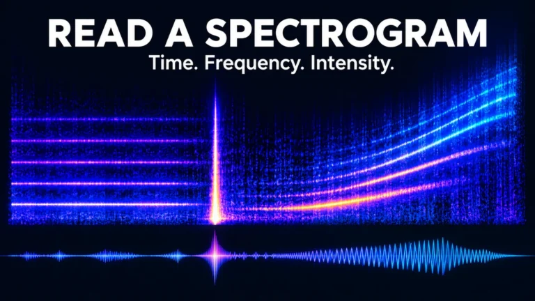
To read a spectrogram, locate time on the horizontal axis, frequency on the vertical axis, and the scale that maps signal strength to brightness or color. Then describe how a feature changes across those dimensions. A horizontal line, a vertical burst and a rising curve answer different questions about the sound.
A spectrogram is a calculated view of an audio signal, not a photograph of its source. Its appearance depends on the recording and the analysis settings. Learning to separate a visible feature from an explanation for that feature is the difference between useful audio observation and confident misinterpretation.
Read the legend before interpreting the picture
Start at the bottom edge. Time usually increases from left to right, but confirm the units and the displayed interval. A panel showing two seconds gives a short click much more horizontal space than a panel showing two minutes. The apparent width of a feature is not a duration until you consult the axis.
Now inspect the vertical axis. Frequency is usually labeled in hertz or kilohertz. One kilohertz is 1,000 cycles per second. A higher position generally means a higher frequency, not a louder event. A faint high-frequency feature can sit above a strong low-frequency feature without being the dominant sound.
Finally find the intensity key. Some displays use bright colors for stronger components; others use darker shades. The Praat spectrogram introduction, for example, describes a grayscale display in which darker areas indicate higher energy density. Do not transfer a color convention from one application to another.
The scale can be relative, normalized or tied to a specified reference. A bright region is not automatically a measurement of acoustic loudness in the room. Microphone sensitivity, recording gain and display processing stand between the physical sound and the plotted value. Read the reference before attaching units or comparing brightness across recordings.
How it differs from a waveform
A waveform plots signal amplitude against time. It helps you locate pauses, peaks and abrupt changes in the recorded samples. A spectrogram distributes information across frequency as time advances. Two sounds can have broadly similar waveform envelopes while containing very different frequency structures.
Imagine a steady low tone and a steady higher tone recorded at similar levels. Their waveform views can both occupy a similar vertical range. In a spectrogram, their bands occupy different frequency positions. If the tone rises gradually, its path moves upward while time continues to the right.
Use both views rather than treating one as a replacement for the other. A waveform can help inspect an abrupt sample-level event; the spectrogram can show whether it affects a narrow band or a broader region. Listening adds another perspective, provided you keep playback at a safe, comfortable level.
iZotope’s spectrogram tutorial illustrates axes and common audio features. Its repair-product suggestions are not needed to understand the display. Seeing a pattern and choosing an editing operation are separate tasks; do not modify the source merely because a graphic looks untidy.
Learn the shapes without turning them into diagnoses
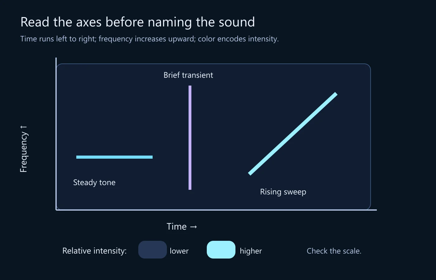
Horizontal bands: sustained frequency components
A stable narrow-frequency component can form a horizontal band. Several regularly spaced bands can indicate a harmonic structure: components related to multiples of a fundamental frequency. That pattern is useful to describe, but it does not uniquely identify a person’s voice, a device or a location.
Measure the spacing using the axis rather than count the apparent pixels. A logarithmic frequency display spreads equal ratios differently from a linear one. Bands that look evenly spaced in one view can look differently arranged in another without any change to the underlying audio.
A persistent low-frequency band might be consistent with hum, but a horizontal line alone does not establish its source. A machine tone, a musical component or another periodic signal could be relevant. Listen to the interval, inspect related bands and retain the uncertainty about the physical cause.
Vertical features: brief events spread across frequency
A short transient can occupy a narrow time region across many frequencies, producing a vertical-looking feature. A click, impact or abrupt edit can contribute such a shape. Their shared appearance is exactly why you should describe the event before naming what produced it.
Zoom in and compare the waveform at the same position. Check whether the feature remains narrow under different appropriate analysis windows. A broad smeared column in a long-window display is not necessarily a physically long sound. The calculation combines information over an interval.
Curves and slopes: frequency changes over time
A rising tone can trace an upward curve; a falling tone can trace a downward one. Speech and many natural sounds contain more complicated moving structures. Begin with the readable statement—frequency increases across this interval—before guessing whether the cause is a siren, a person or processing.
A sloping line also needs the actual time and frequency scales to be compared with another example. Enlarging the horizontal axis makes the slope appear flatter. A screenshot’s geometric angle is not an application-independent measurement of the rate of frequency change.
Diffuse regions and gaps
Broadly distributed energy can appear as a textured cloud rather than a tidy line. A dark region may indicate low displayed energy, a thresholded part of the signal or an actual gap. The palette and dynamic range influence how much low-level material remains visible.
Do not equate black with digital silence unless the data and settings support that conclusion. A display can hide quieter components below its lower limit. Conversely, raising the display sensitivity can reveal structure without showing that the recording suddenly acquired additional sound.
Scales and analysis settings change the view
A frequency-axis check can be as simple as reading three tick marks. On a linear axis, the interval from 1 to 2 kHz takes the same vertical distance as 2 to 3 kHz. On a logarithmic axis, equal ratios receive equal distances: 1 to 2 kHz occupies the same distance as 2 to 4 kHz. This changes how harmonic spacing looks even when the analyzed values are identical.
Before comparing two screenshots, find a frequency you can identify on both axes and inspect the same neighborhood. Do not stretch one image until the lines seem to match; image scaling can conceal the differing coordinate systems. If the display has no readable axes or settings, treat it as a qualitative illustration of shape rather than a basis for a numerical comparison.
Many spectrograms are built by applying a short-time Fourier transform. The analysis repeatedly considers a windowed interval of the signal, computes its frequency content and moves the window forward. Each column is therefore a summary over an interval, not an instantaneous reading at one infinitely precise moment.
A longer analysis window generally distinguishes nearby frequency components better but localizes brief timing changes less precisely. A shorter window can make transients easier to place in time while separating close frequencies less clearly. There is no single best setting for every question.
Separate window length from how often windows are evaluated. Increasing overlap can make the display more finely sampled in time, but it does not undo the information mixed within each window. More columns do not automatically mean that the sound’s events have become independently resolved at that finer spacing.
The SciPy ShortTimeFFT documentation makes these parameters explicit: window, hop, sampling frequency and FFT length play different roles. Its definitions are useful even if you use a graphical application rather than write analysis code.
A numerical example with stated assumptions
Assume audio sampled at 48,000 samples per second. A window containing 1,024 samples spans approximately 21.33 milliseconds. With an unpadded 1,024-point FFT, the frequency-bin spacing is 48,000 / 1,024, or 46.875 hertz. Those calculations describe the chosen analysis, not a measured sound event.
A 4,096-sample window spans approximately 85.33 milliseconds, and an unpadded 4,096-point FFT has bins spaced about 11.72 hertz apart. It gathers information across a longer interval. This can be useful for closely spaced steady components, while a short click’s timing may become less sharply localized in the view.
Bin spacing is not a complete definition of resolving power. The window’s shape and duration matter. Padding a short window with zeros can provide more plotted frequency points without collecting a longer observation. Do not report the resulting finer-looking grid as proof that two previously unresolved tones are now independently resolved.
A reading exercise: describe three events before naming them
Consider a designed display with three features: a steady band across the first second, a brief vertical feature near the middle, and a rising band later. The explanatory image provides a simplified map of those shapes. It does not claim to identify a particular recording or reproduce a measured incident.
For the first feature, write its time interval and approximate frequency range from the actual axes of the display you are using. Add whether related bands are visible. “A narrow component persists through this interval” is a sound observation. “The room contains this exact electrical device” requires additional evidence.
For the vertical feature, locate the corresponding waveform interval and listen at a comfortable level. Describe its duration only to the precision the analysis supports. If it looks wider in the long-window view, do not treat the width difference as a change in the file. You changed the measuring view.
For the rising feature, record the starting and ending frequency ranges and the interval over which the rise occurs. Keep the source channel and display settings with the note. A curve traced from a screenshot without scale information is a visual description, not a reproducible frequency measurement.
Only then consider possible sources or processing explanations. The order matters: an early label can make you interpret every later detail as confirmation. A settings-aware observation stays useful even when the first hypothesis turns out to be wrong.
Build a comparison that does not compare settings by accident
Use the same audio version, channel and interval for an initial comparison. Record the sampling rate, window type and length, hop or overlap, FFT size, frequency scale and intensity range where the application exposes them. Not every tool uses the same terminology, so preserve the relevant settings rather than force them into guessed equivalences.
Then vary one analysis setting to test a specific question. A shorter window can help examine when a transient occurs; a longer one can help inspect a sustained low-frequency component. Keep both views and explain why they differ. Do not choose only the view that makes an artifact look most suspicious.
For two different recordings, match the display conditions where appropriate, but also note recording differences. Gain, microphone response, channel mixing and compression can change the visible energy. Equal palettes do not make two recording paths identical.
Automatic scaling deserves special attention. If a program adjusts the intensity reference to the visible interval, scrolling can change the darkness of material that did not change. Praat’s documentation explains such a display behavior. A before-and-after screenshot must therefore retain enough settings information to show what was actually held constant.
| Item | Reason | Common mistake |
|---|---|---|
| Source version and channel | Identifies the signal examined | Comparing a mono mix with one original stereo channel |
| Time and frequency ranges | Makes coordinates meaningful | Interpreting a screenshot’s slope without scales |
| Window and FFT settings | Explains resolution and smoothing | Treating finer plotted bins as new signal information |
| Intensity scale and reference | Controls visible contrast | Calling a dark area absolute silence |
Video audio brings its own version history
A video platform may deliver audio that has been encoded, mixed or otherwise processed. Extracting that track into another format does not restore what the microphone originally recorded. Keep the supplied video and label an extracted track by its source version.
When an audio event is being compared with a visible action, align the event carefully. A trim, offset or changed playback speed can make equal displayed timestamps refer to different moments. A spectrogram can locate signal features within its own time axis; it does not automatically establish synchronization with a separate video.
The existing lip-sync discussion concerns audiovisual relationships. This article does not replace it with a frequency picture. A visible burst may help choose an interval to review, but it is not proof that a particular mouth movement produced that sound.
Keep channels separate initially when their distinction matters. Combining channels can change their content through addition and cancellation. A narrow feature missing from a mix may remain in an individual channel. Document the operation before interpreting its result as an event disappearing from the original recording.
A spectral feature is not a deepfake detector
Synthetic speech, edited recorded speech and ordinary captured audio can share many visible structures. A cutoff, smooth region or unusual harmonic pattern is not a universal signature of cloning. Recording and delivery conditions can create or obscure similar features.
Likewise, a detailed natural-looking spectrogram does not establish who spoke or whether the words were edited. Identity, source history and content integrity require additional evidence. The existing voice-deepfake guide addresses the wider assessment; do not substitute a visual impression for that work.
If you encounter an unexplained feature, preserve its coordinates and the source. State plausible alternatives without assigning unsupported probabilities. A specialist may need the original recording and a validated method to answer a consequential authenticity question. A screenshot can communicate a location of interest, but it cannot carry every analytical detail.
Use the display to ask a better next question
A narrow sustained band suggests asking whether a stable tonal component is audible and whether it appears in the surrounding interval. A brief broadband feature suggests checking a local waveform event. A change across an edit suggests comparing source versions and timing. These are specific next questions, not labels that settle a file’s origin.
For repair work, keep the received recording and create a separate edited copy. Removing an unwanted feature can improve listening, but it changes the material you are examining. Do not use a cleaned rendition as though it preserves every feature of the original track.
For a review handoff, combine a short observation with source identity, channel, interval and analysis settings. “Brief broadband event near the stated position, visible under both chosen windows; cause not established” is more useful than “suspicious spike.” The former gives another person a way to continue without inheriting your assumption.
Common reading questions
Does the highest visible frequency determine audio quality?
No. A frequency limit can reflect recording, processing or display settings, while useful quality also depends on noise, distortion, intelligibility and purpose. A broad visible range is not proof of an unprocessed source. Check what the file and analysis actually represent.
Can a spectrogram show the exact cause of a click?
It can show a short event’s frequency distribution within the analysis limits. Several physical and processing causes can produce similar shapes. Use listening, waveform inspection and the recording context to investigate rather than name a cause from the vertical line alone.
Why does the same sound look different in another application?
The tools may use different windows, scales, references, colors or normalization. Start by comparing their settings and the exact source interval. A display difference is not evidence that the sound file changed. The video forensics framework helps keep analytical representations distinct from source evidence.
Read coordinates first, settings second and causes last. That habit turns a visually impressive graphic into a useful account of what is in the supplied signal—and keeps its limits as readable as its brightest features.
Technical references
- Praat: Viewing a spectrogram — axes, intensity convention and view-dependent behavior.
- iZotope: Spectrograms explained — common shapes and the time-frequency tradeoff.
- SciPy: ShortTimeFFT — window, hop, sampling frequency and FFT-bin definitions.
- SciPy signal-processing tutorial — spectral analysis and short-time transforms.
The 48 kHz window calculations are derived directly from the stated parameters; no new audio experiment or detector result is claimed.